Engineering story
Chapter 9 · Beam-Columns
Beam-column design with second-order effects, B1/B2 factors.
A real project narrative for this chapter will be authored as this chapter migrates to the v3.0 structured schema.
Beam-column design with second-order effects, B1/B2 factors.
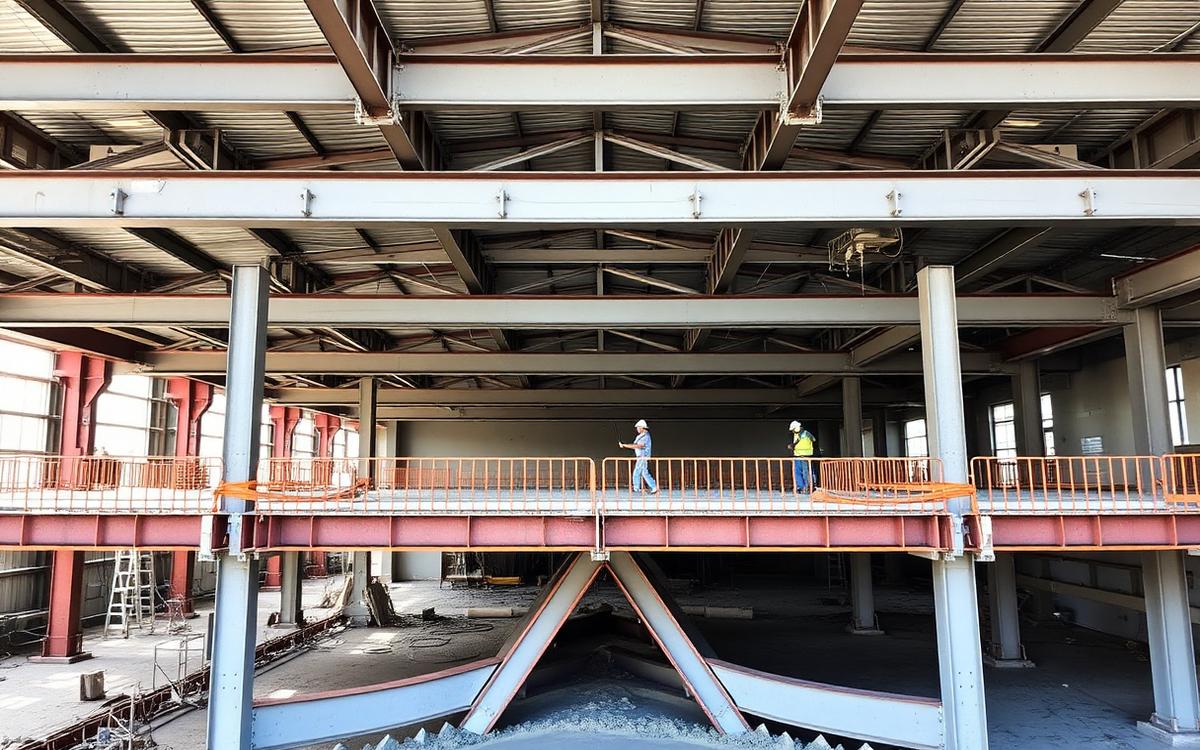
Beam-column design with second-order effects, B1/B2 factors.
A real project narrative for this chapter will be authored as this chapter migrates to the v3.0 structured schema.
Photographs and lessons-learned case studies for this topic will be added during chapter migration.
Sway frames experience P-Δ (structure-level) and P-δ (member-level) second-order effects. Ignoring these gives moments that can be 20–50% too low, leading to premature buckling.
Foundational for Chapter 17 stability and every moment-resisting column in Chapters 19–20.
Use this reference to flip directly to the correct page of the AISC 360-22 Specification while solving problems in this course chapter.
| § | Section title | Page |
|---|---|---|
| C1 | General Stability Requirements | 16.1-15 |
| C2 | Calculation of Required Strengths (Direct Analysis Method) | 16.1-16 |
| C3 | Calculation of Available Strengths | 16.1-19 |
| H1-1a | Interaction Eq. (Pr/Pc ≥ 0.2) | 16.1-114 |
| H1-1b | Interaction Eq. (Pr/Pc < 0.2) | 16.1-114 |
| App. 8 | Approximate Second-Order Analysis (B1, B2 Amplifiers) | 16.1-235 |
Companion reference: AISC Manual Part 6 & Appendix 8
A beam-column is any member subjected simultaneously to axial force Pr and flexural moment Mr about one or both axes. Every perimeter moment-frame column, every column with an eccentric crane bracket, and every truss chord with panel-point transverse load is technically a beam-column. AISC does not have a separate "beam-column chapter" for capacity — instead Chapter H combines the axial capacity (Ch. E) and flexural capacity (Ch. F) you already computed with an interaction equation.
A first-order analysis computes forces and moments on the undeformed geometry — the standard linear-elastic stiffness method every student learns first. A second-order analysis re-equilibrates the structure on its deformed shape, so that axial forces acting through lateral displacements generate additional moment that a first-order analysis misses entirely.
B1 scales up the "no-translation" moment Mnt (the moment from a gravity/braced analysis with sidesway artificially restrained) to account for P-δ along the member:
Physically: B1 is how much larger the true mid-span moment becomes because axial load is now acting on a bowed shape rather than a straight one. As Pr approaches the member's own Euler load Pe1, the denominator shrinks toward zero and B1 blows up — this is the mathematical signature of buckling instability.
Cm corrects for the fact that Pe1 was derived for a member bent into a single half sine wave under uniform moment. Real end-moment diagrams are rarely that shape, so Cm "reduces" the amplifier when the real moment diagram is less severe than uniform single curvature.
If B2 exceeds ~1.5 the structure is dangerously flexible and Appendix 8's linear approximation of instability is no longer trustworthy — stiffen the frame (larger columns, added bracing) rather than trusting the amplifier further.
Subscript nt = "no translation" (a gravity-only analysis with joints artificially restrained against sidesway); lt = "lateral translation" (a pure sidesway analysis under lateral load, or notional load). Two separate first-order analyses are run, then combined with the amplifiers above — you never need to run an actual second-order computer analysis to use this method.
There are two accepted design paths in AISC 360-22 for stability:
DAM (Chapter C) is now the AISC-preferred default: it removes the alignment-chart K-factor step entirely (always K = 1.0) by instead explicitly modeling frame out-of-plumbness (notional loads) and inelastic softening (0.8τbEI). ELM (Appendix 7) is still permitted, and is what most legacy problem sets — including Examples E.4A/E.4B in this chapter — use, via the sidesway alignment charts.
Both equations describe a single design envelope in Pr–Mr space: a straight line above Pr/Pc=0.2, transitioning to a shallower straight line below it (so the moment term is not over-penalized for lightly-loaded columns). §H2 provides an alternative, point-by-point stress-ratio check that is less conservative when it applies (both axial and flexural stress computed at the same fiber) — see Worked Example 9.1.
AISC Manual Table 6-2 tabulates φPn, φMnx, φMny, and the H1-1 combined-stress coefficients directly by shape and unbraced length — it turns the whole H1 check into a lookup-and-multiply exercise. Manual Table 6-1 (used in Examples H.2 and H.4) instead tabulates available stresses Fca, Fcbx, Fcby for the §H2 stress-ratio method.
Companion reference: Manual Part 6 (Table 6-2) + Appendix 8 / Chapter C (B1/B2 amplifiers). In practice, engineers rarely compute every quantity from first principles — the AISC Steel Construction Manual (16th Ed.) tabulates φRn (or Rn/Ω) for every rolled shape so you can pick a member in seconds. Formulas remain essential for understanding, verifying, and for anything the tables do not cover.
The Manual tables assume K=1.0 (Direct Analysis Method) and require you to enter amplified Mr = B1·Mnt + B2·Mlt. Compute B1, B2 by hand (Chapter C), then use Table 6-2 exactly as for the H1.1 check above.
Common shortcut: if the frame is braced and reverse-curvature (Cm ≤ 0.6, α Pr/Pe1 < 0.05), B1=1.0 exactly and no amplification is required — go straight to Table 6-2.
Every chapter's worked example is one step in the design of the same building: Plan: 4 bays N–S × 3 bays E–W, each 30 ft × 30 ft. Stories: 4 @ 13 ft (52 ft roof). Composite floor: 4.5 in NW concrete on 3 VLI20 deck. Roof: 1.5 in B-deck + insulation + membrane. Materials: Wide-flange members A992 (Fy = 50 ksi, Fu = 65 ksi). Plates A572 Gr. 50. HSS bracing A500 Gr. C. Bolts A325-N 7/8 in dia. Welds E70XX. Concrete f'c = 4 ksi. Anchor rods F1554 Gr. 36.
| Name | Equation | AISC Ref |
|---|---|---|
| Interaction (Pr/Pc ≥ 0.2) | Pr/Pc + (8/9)(Mrx/Mcx + Mry/Mcy) ≤ 1.0 | AISC §H1.1(a) |
| Interaction (Pr/Pc < 0.2) | Pr/(2 Pc) + (Mrx/Mcx + Mry/Mcy) ≤ 1.0 | AISC §H1.1(b) |
Adapted from AISC Design Examples V16.0, Example H.4
Problem statement. Select an A992/A992M W-shape of 10 in. nominal depth to carry axial compression of 5 kips dead + 15 kips live. The unbraced length is 14 ft, ends are pinned, and the frame is not subject to sidesway. The member also carries moments from uniformly distributed loads, not including second-order effects:
Engineering interpretation: B1x = 1.02 but B1y = 1.09 — the weak axis is nine times more sensitive to P-δ because Pe1y is only 371 kips while Pe1x is 1,734 kips. Amplification is not driven by how big the axial force is, it is driven by how close it gets to the elastic buckling load about the axis you are bending about. Also note the answer is 0.979: skipping the B1 amplification entirely would have given about 0.960 and hidden the fact that this member is essentially at capacity.
Problem statement. A typical story of a moment-frame office building is 13 ft (156 in.) tall. Under the LRFD lateral load combination, the story carries a total gravity load of ΣPstory = 3,600 kips, the story shear is H = 120 kips, and a first-order analysis gives a story drift of ΔH = 0.45 in. A particular column in that story has first-order results Pnt = 240 kips, Plt = 60 kips, Mnt = 45 kip-ft, Mlt = 180 kip-ft, with B1 = 1.00. Determine the second-order required strengths using the amplified first-order method.
Engineering interpretation: B2 is a story property, not a member property. Every column in the story gets the same B2 because they all sway together. That is also why stiffening one column reduces the amplification for all of them, and why the fastest way to bring B2 down is to stiffen the story (reduce ΔH), not to enlarge one member.
Adapted from AISC Design Examples V16.0, Example E.4A
Problem statement. In the moment frame shown, sidesway is uninhibited in the plane of the frame. Column B-C is an A992 W14×82, 14 ft long, continuously braced about its y-y axis, with the base fixed about x-x. Roof girders are W18×50 (Ix = 800 in⁴) and floor girders are W24×55 (Ix = 1,350 in⁴), each spanning 35 ft. Column loads at B-C are PD = 41.5 kips and PL = 125 kips. Determine whether the column is adequate.
Engineering interpretation: K = 1.85 for a sway column means the column behaves as if it were 85% longer than its physical height. If you had (incorrectly) used K = 1.0, Lc/r would be 27.8, Fcr would be about 46 ksi, and you would overestimate capacity by roughly 12%. In real moment frames K values of 1.5–2.5 are routine, which is precisely why the Direct Analysis Method — where K is always 1.0 — is now the AISC default.
Problem statement. The same frame is now to be analyzed by the AISC §C2 Direct Analysis Method. The level under consideration carries a total factored gravity load Yi = 1,800 kips. Determine the notional load, the analysis stiffnesses, and the effective length to be used in the strength check. The W14×82 column carries Pr = 250 kips.
Engineering interpretation: the two methods look like they give very different answers, but they don't — they just move the conservatism. DAM reports a larger available strength (1,022 vs 890 kips) because K = 1.0, and pays for it with larger required strengths from a deliberately softened, deliberately out-of-plumb model. ELM keeps the analysis "honest" and buries the stability penalty in K. Never mix them: a K = 1.85 check on DAM forces is doubly conservative, and a K = 1.0 check on nominal-stiffness forces is unconservative and non-code-compliant.
Chapter 8 of the textbook develops beam-column design. AISC §H1 interaction equations combine the axial demand ratio Pr/Pc with bending demand ratios Mrx/Mcx, Mry/Mcy. Second-order effects use B1 (no-translation) and B2 (translation) amplifiers per Appendix 8, or solve via the Direct Analysis Method (Chapter C).
Setup. W12×72, A992, Pu = 400 k, Mux = 200 k·ft, Muy = 0. φcPn = 818 k, φbMnx = 425 k·ft.
AISC Reference: AISC §H1.1
Interaction ratio?
Pr/Pc = 400/818 = 0.489 ≥ 0.2 → H1-1a: 0.489 + (8/9)(200/425) = 0.489 + 0.418 = 0.91 ≤ 1.0 OK.
Setup. Single-curvature: M1 = +60 k·ft, M2 = +120 k·ft; Pu = 250 k; Pe1 = 2400 k.
AISC Reference: AISC App. 8
B1?
Cm = 0.6 − 0.4·(60/120) = 0.4. B1 = 0.4/(1 − 1.0·250/2400) = 0.4/0.896 = 0.446 < 1 → use B1 = 1.0; for opposite-curvature inputs (M1/M2 = −0.5) Cm = 0.8 → B1 = 0.893/0.896 ≈ 1.05.
Setup. Story gravity ΣPnt = 1800 k; story buckling sum ΣPe2 = 12,000 k; α = 1.0 (LRFD).
AISC Reference: AISC App. 8
B2?
B2 = 1/(1 − 1.0·1800/12000) = 1/0.85 = 1.176.
Each example mirrors the NCEES FE Civil Reference Handbook style: brief givens, a labeled figure, AISC section reference, step-by-step numeric solution, and a single boxed answer.
These questions reference AISC Steel Construction Manual (16th ed.) — sections, equations, and tables are cited explicitly. Use a calculator. Each question offers a clue you may reveal before answering. Submissions are recorded to your account once signed in.
Attach your handwritten or typed step-by-step solution for this chapter's graded quiz. The instructor can download every submission. PDF only, up to 25 MB.
Your file — PDF, Word document, scanned handwriting or a photo — is read page by page like an experienced structural engineering instructor would. The scan is validated first, then your reasoning, structural model, calculations, diagrams, code basis and final answers are graded on process, not just the final number. Design work is additionally reviewed against AISC 360-22 and ACI 318-19. Partial credit applies, and one early mistake carried correctly forward is only penalized once.
Calculator tips coming soon.
Traps coming soon.
Aim for ~3 minutes per FE problem; skip and return to any item that takes longer than 5 minutes.