Engineering story

A century of steel — from concept to skyline

Engineer reviewing blueprints against a steel-frame construction site at sunrise

Almost every real column is a beam-column.

AISC 360-22 Chapter H closes the loop: axial + biaxial bending in a single interaction equation, with second-order (B1, B2) amplification.

Chapter 8 covers AISC 360-22 Chapter H: the H1-1a / H1-1b interaction equations, second-order amplification B1 (member) and B2 (story sway), the Cm reduction factor, and how to combine them into a code-compliant beam-column check.

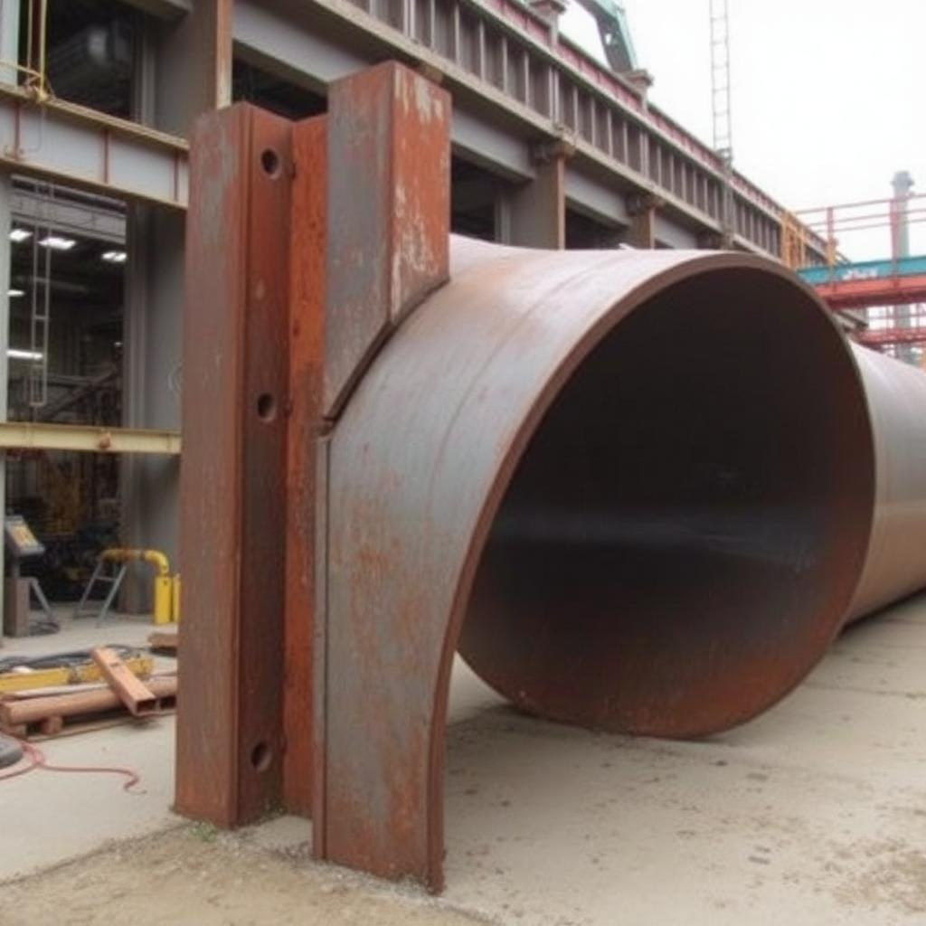
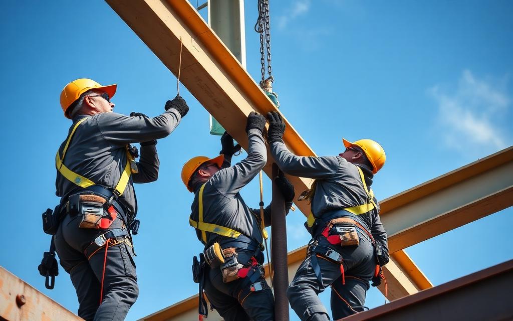
Iconic steel structures built on engineering excellence

AISC ASD interaction (fa/Fa + fb/Fb)
1963
LRFD H1 introduced
1986
AISC 360-05 direct analysis method (DAM)
2005
AISC 360-22 Chapter H (current)
2022

Load pathRoof/floor gravityWind momentColumn axial + momentBase plateFoundation

02

Learning objectives

What you will be able to do after finishing Chapter 1 — and why each objective matters in practice

Objective 01

Apply H1-1a (Pr/Pc ≥ 0.2)

Pr/Pc + (8/9)(Mrx/Mcx + Mry/Mcy) ≤ 1.0 governs when axial is the primary demand.

Why it matters: Most gravity columns fall here; a single line captures failure.
Where it is used: Interior gravity columns in moment frames.
Connects to: AISC H1.1a.

Objective 02

Apply H1-1b (Pr/Pc < 0.2)

Pr/(2Pc) + (Mrx/Mcx + Mry/Mcy) ≤ 1.0 governs when bending dominates.

Why it matters: Perimeter/moment-frame columns with light axial load.
Where it is used: Perimeter moment-frame columns.
Connects to: AISC H1.1b.

Objective 03

Compute B1 amplifier

B1 = Cm / (1 − α·Pr/Pe1) ≥ 1.0, applied to non-translation moments Mnt.

Why it matters: Captures P-δ effect on member curvature.
Where it is used: Every beam-column when second-order effects are non-negligible.
Connects to: AISC App. 8; C2.1(b).

Objective 04

Compute B2 sway amplifier

B2 = 1 / (1 − α·Pstory/Pe,story) applied to lateral-translation moments Mlt.

Why it matters: Captures P-Δ story sway in moment/braced frames.
Where it is used: Story-level analysis of moment frames.
Connects to: AISC App. 8; C2.1(b).

Objective 05

Select Cm for the load pattern

Cm = 0.6 − 0.4(M1/M2) for members without transverse loads between supports; Cm = 1.0 otherwise (conservative).

Why it matters: Reverse curvature reduces B1; single curvature increases it.
Where it is used: Every B1 calculation.
Connects to: AISC App. 8.2.1.

Objective 06

Read Manual Table 6-2 (φPn, φMnx)

Table 6-2 collects φPn and φMn for common W-shapes — the fastest H1 check.

Why it matters: Turns a full beam-column check into two lookups + one line.
Where it is used: Every gravity/wind column check in practice.
Connects to: AISC Manual Part 6.

03

Engineering motivation

What each part of a steel-frame building actually does — and why it exists

Before you design any single member, you have to see the whole system. A steel-frame building is not a collection of independent shapes bolted together — it is a deliberate load path, engineered so that every kilonewton of gravity, wind, or seismic demand has a continuous route from where it starts to the ground where the earth can resist it.

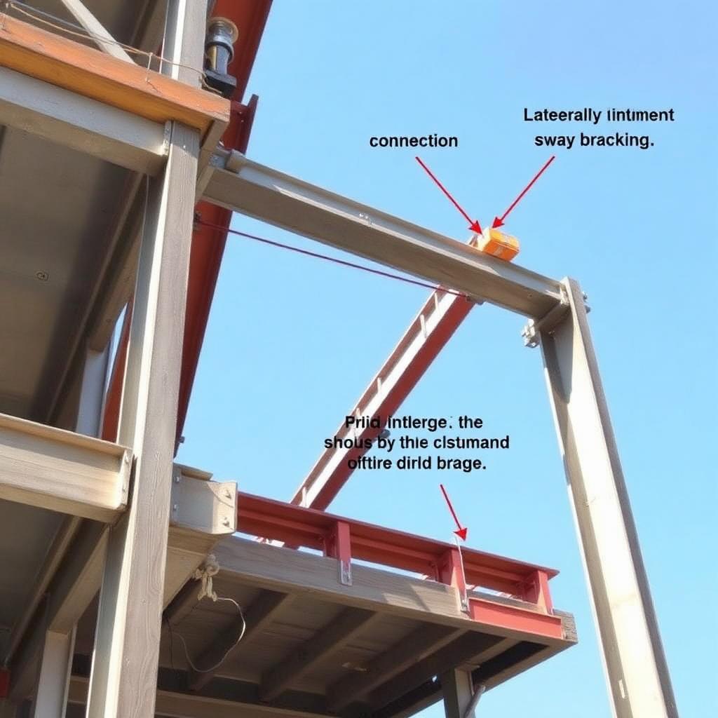
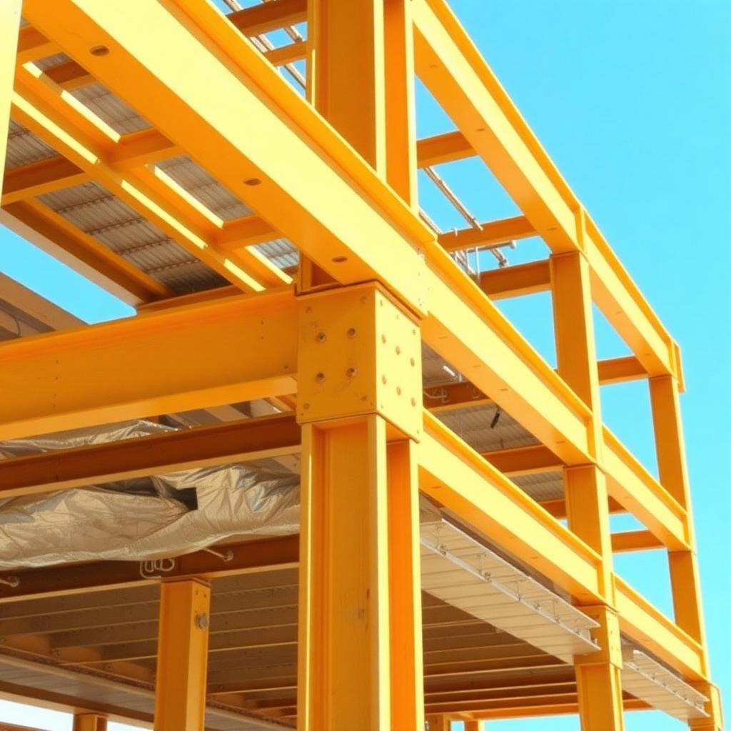
The photograph below shows a typical steel framing detail. Drag each labelled chip onto the structural element it names — the drop is only accepted when it lands inside the correct element's outlined region. A correct answer locks in with a green outline and a short explanation; a wrong answer flashes the region red, tells you what you actually hit, and returns the chip so you can try again. Press Reveal expected placements to see the reference solution (that attempt is then marked as assisted).

Structural steel framing — identify each element by dragging the labels — Fig. 1.3 · Drop a chip inside the outlined element it names. Green = correct and locked; red flash = wrong element, chip returns.

04

Failure mechanisms

Why we design the way we do — six ways steel structures have failed, and what each disaster taught the profession

Every provision in AISC 360 is a scar. Behind each equation, load factor, and detailing rule is a bridge, a walkway, or a tower whose failure cost lives and rewrote the profession. The six case studies below trace the mechanisms that motivate the code you are about to learn.

Read each one as an engineer, not a spectator: identify the load, the limit state, the missing check, and the specific clause that exists today because that check was missed. When you meet those clauses again in Chapters 5–17, they will read as answers, not rules.

Failure mechanism

In-plane interaction collapse

The column reaches the H1-1a envelope — plastic hinge forms as P and M both climb.

Root cause

Pr/Pc + (8/9)(Mr/Mc) exceeds 1.0.

Lesson learned

Either upsize the shape or reduce Mr via bracing / stiffer frame.

§AISC H1.1a

Failure mechanism

Out-of-plane LTB of beam-column

Column buckles laterally out-of-plane before H1-1a is reached because Mcy governs.

Root cause

Lb too long about the weak axis; Mn drops.

Lesson learned

Add weak-axis bracing to raise Mcy and unlock H1.

§AISC H1.3 / F2

Failure mechanism

P-Δ sway instability

Story drift amplifies moments until B2 → ∞.

Root cause

α·Pstory / Pe,story approaches 1.0.

Lesson learned

Increase story lateral stiffness (bracing / larger columns).

§AISC App. 8 / DAM C2

How failure propagates

The five-stage failure progression

1Gravity axial

2Add wind moment

3B1/B2 amplification

4Reach H1 = 1.0

5Plastic hinge / sway collapse

Design codes intervene at the transition from yield to instability. Everything before yield is elastic and reversible; everything after instability is a race to collapse. LRFD keeps the demand well below the first transition.

05

Lecture notes

The full textbook chapter — figures, equations, and engineering narrative

Reflection · Think before you read

A column in a moment frame carries axial gravity load plus wind moment. Why isn't it safe to check axial and bending separately and add the demand/capacity ratios? What does the AISC interaction equation capture that a simple sum misses?

Chapter 8 — Combined Axial Load and Bending (AISC 360-22 Chapter H)

Chapter focus. No real steel member sees pure axial load or pure bending in isolation — gravity eccentricity, wind, and seismic drift all add moment to a column, and every beam-column in a moment frame must resist both simultaneously. AISC Chapter H does not re-derive new strength equations; instead it takes the axial capacity you already know from Chapter E and the flexural capacity from Chapter F and combines their demand-to-capacity ratios in a single interaction inequality. Get comfortable with H1's two-branch equation, and you can handle 95% of beam-column checks you will ever see.

1. The Interaction Concept

Imagine a column loaded with only axial force P: it fails at P_n. Now imagine it loaded with only moment M: it fails at M_n. If you apply both P and M simultaneously, the member fails at combinations of P and M that lie somewhere between these two extremes — the member is "using up" part of its strength budget on each effect, and the two shares must sum to no more than the total available strength. AISC's interaction equations are a straight-line (linear) or piecewise-linear approximation to the more complex actual failure surface (which is slightly convex for compact wide-flange members), calibrated to be safe and reasonably efficient across the practical range of proportions.

2. Required vs. Available Strengths — Get the Sides Right

Before writing any interaction equation, be crystal clear about which numbers go on which side. The required strengths P_r, M_rx, M_ry are the factored (or ASD) demands acting on the member, and critically, per Chapter C, they must already include second-order effects (P-δ member curvature and P-Δ sidesway) — Chapter H itself does not amplify anything. The available strengths φP_n, φM_nx, φM_ny (or P_n/Ω, M_n/Ω) come straight from Chapter E (compression) and Chapter F (flexure) for the trial shape, unbraced length, and bracing pattern being checked.

Figure 8.1 — Required strengths (2nd-order analysis) on one side, available strengths (Ch. E / Ch. F) on the other; H1 is the bridge between them.

3. AISC H1.1 — The Two-Branch Interaction Equations

§H1.1 covers doubly- and singly-symmetric members subject to axial force and bending about one or both principal axes. The branch you use depends entirely on how large the axial demand ratio is relative to axial capacity:

Decision box — which H1 equation applies?

Compute the axial demand ratio P_r/(φP_n) (or P_r/(P_n/Ω) for ASD).
If ≥ 0.2 → use H1-1a (axial-dominated branch, moment terms scaled by 8/9).
If < 0.2 → use H1-1b (moment-dominated branch, axial term halved).
Biaxial bending? Both M_rx/φM_nx and M_ry/φM_ny appear together in the same equation — never check the two axes separately and add pass/fail results.
At exactly P_r/φP_n = 0.2 the two equations give identical results by construction — this is a deliberately continuous, kinked envelope, not two competing formulas.

Figure 8.2 — Two-part linear/8-9-slope H1 envelope; the kink occurs at P_r/φP_n = 0.2.

H1-1a: Pr/(φPn) ≥ 0.2

(1)

P_{r} / (ϕ P_{n}) + (8/9) \cdot [M_{r x} / (ϕ M_{n x}) + M_{r y} / (ϕ M_{n y})] \leq 1.0

H1-1b: Pr/(φPn) < 0.2

(2)

P_{r} / (2 \cdot ϕ P_{n}) + [M_{r x} / (ϕ M_{n x}) + M_{r y} / (ϕ M_{n y})] \leq 1.0

P_r = required (2nd-order) axial strength, compression or tension.
P_c = φ_cP_n (compression, Ch. E) or φ_tP_n (tension, Ch. D).
M_rx, M_ry = required (2nd-order) flexural strengths about the strong and weak axes.
M_cx = φ_bM_nx, M_cy = φ_bM_ny from Chapter F, using the actual L_b and C_b for the member.

Physically: the 8/9 factor in H1-1a reflects that at high axial load the plastic P-M interaction surface curves inward slightly from a straight line, so a straight line alone would be unconservative; multiplying the moment terms by 8/9 corrects for this while keeping the equation linear and easy to use by hand.

4. Why Pr/Pc = 0.2 Is the Threshold

The 0.2 threshold is not arbitrary — it is where the exact nonlinear plastic interaction surface for a typical doubly-symmetric wide-flange shape is best approximated by switching from one straight-line segment to another. Below 0.2, axial load has a comparatively small effect on the available moment capacity of the section (for compact members not controlled by LTB, the plastic moment is not much reduced by low axial load), so it is conservative-but-not-overly-conservative to simply halve the P_r/P_c term. Above 0.2, axial load significantly reduces the effective plastic modulus available for bending, so the moment terms need the 8/9 penalty to stay safe.

5. The Role of C_m and Second-Order Amplification

The moments M_rx, M_ry plugged into H1 must already be amplified for P-δ and P-Δ effects — Chapter H assumes this work is already done. Historically (and still commonly taught alongside Chapter H), the classic B₁/B₂ amplifier method computes:

(3)

M_{r} = B_{1} \cdot M_{n t} + B_{2} \cdot M_{l t}, B_{1} = C_{m} / (1 - α P_{r} / P_{e 1}) \geq 1.0

where C_m is an equivalent-uniform-moment factor that accounts for the actual (often non-uniform) moment diagram along the unbraced length — for a member bent in reverse curvature (no transverse load between braced points), C_m = 0.6 − 0.4(M₁/M₂), where M₁/M₂ is negative for reverse curvature (a lower, more favorable C_m) and positive for single curvature. For members with transverse load between supports, C_m = 1.0 is conservative unless a more refined value is derived. The full B₁/B₂/C_m derivation and worked amplification examples are developed in Chapter 9; for this chapter, treat P_r and M_rx, M_ry as already-amplified inputs to H1.

Modern practice increasingly uses the Direct Analysis Method (Ch. C), which captures second-order effects directly in the structural analysis (reduced stiffness + notional loads) rather than through B₁/B₂ amplification of a first-order analysis — see Chapter 17.

6. Biaxial Bending — One Equation, Not Two

When a column has moment about both axes (typical of corner and edge columns in a moment frame under two-way wind or seismic loading), both M_rx/M_cx and M_ry/M_cy appear as an additive sum inside the same bracket of H1-1a/1b. This means a column that easily passes strong-axis bending alone and easily passes weak-axis bending alone can still fail the combined check — the interaction is not "worst axis governs," it is "both axes add."

Figure 8.3 — Biaxial bending: M_rx and M_ry ratios sum together against the same interaction envelope, not evaluated independently.

7. H1.2 — Alternative Approach for Doubly Symmetric Members in Flexure and Tension

§H1.2 gives an important, often-overlooked refinement for a doubly symmetric member subject to flexure and axial tension simultaneously (rather than compression). Because axial tension tends to straighten a member and delay lateral-torsional buckling, §H1.2 allows the LTB modification factor C_b computed for flexure alone to be increased using a correction based on the Euler buckling load about the minor axis, P_ey:

Spec. Eq. H1-2 / H1-3

(4)

P_{ey} = π^{2} E I_{y} / L_{b}^{2}

C_{b}^{'} = C_{b} \cdot (1 + α \cdot P_{r} / P_{ey})

where α = 1.0 (LRFD) or 1.6 (ASD), reflecting the different load factor conventions. The resulting larger C_b increases M_n for LTB, recognizing that a tension-braced beam is genuinely stronger against lateral-torsional buckling than the same beam under compression. The H1-1a/1b interaction equations themselves are unchanged — this only affects how M_n (and therefore M_c) is computed going in.

8. §H2 — General Interaction Equation for Unsymmetric and Other Shapes

§H1 assumes the member is doubly or singly symmetric and that its principal bending axes coincide with the geometric x-y axes. For unsymmetric shapes — single angles, WTs bent about a non-principal axis, or any shape where the flexural and torsional/warping behavior couples in a complex way — AISC provides the more general, stress-based §H2 equation, checked at the specific extreme fiber points on the cross-section (not simply "top" and "bottom"):

Spec. Eq. H2-1

(5)

f_{r a} / F_{c a} + f_{r b w} / F_{c b w} + f_{r b z} / F_{c b z} \leq 1.0

Here f_ra, f_rbw, f_rbz are the required axial and flexural stresses (not forces) about the principal w and z axes at the point being checked, and F_ca, F_cbw, F_cbz are the corresponding available stresses. §H2 is more general but also more tedious — always prefer §H1 whenever it legitimately applies (doubly/singly symmetric shape, bending about geometric axes).

Figure 8.4 — §H2 is required for genuinely unsymmetric shapes where principal axes w, z are rotated relative to the geometric x, y axes.

9. §H3 — Members Under Torsion, and Torsion Combined with Other Forces

Torsion is uncommon in typical gravity framing but shows up in spandrel beams, crane girders with eccentric loads, and any member where the load path is offset from the shear center. §H3 requires that the normal stress due to torsional warping (σ_w, for open shapes like W-shapes and channels) be combined linearly with axial and flexural normal stresses at each point of the cross-section, while shear stress due to torsion (τ) combines with flexural shear using a von Mises–type interaction:

Spec. §H3.1 (normal stress, linear combination)

(6)

σ = P / A \pm M_{x} c_{x} / I_{x} \pm M_{y} c_{y} / I_{y} \pm σ_{w} \leq F_{y} /Ω or ϕ F_{y}

Spec. Eq. H3-6 (shear stress combination)

(7)

(f_{v}^{2} + 3 f_{t}^{2}) \leq 0.6 F_{y} /Ω or ϕ (0.6 F_{y})

Closed shapes (HSS) have high torsional stiffness (large St. Venant constant J) and negligible warping, so §H3.2 gives a much simpler check using only the torsional shear stress; open shapes (W, C, single angles) can develop significant warping normal stress that must be tracked separately. Full torsion analysis (computing σ_w and warping section properties) is beyond the scope of most introductory courses but the concept — torsion adds another stress term that must be superimposed, not treated independently — is essential.

Figure 8.5 — §H3 overview: normal (warping) stress adds linearly; shear stresses combine using a von Mises-type square-root-sum-of-squares rule.

10. Preliminary Sizing — Manual Tables 6-1/6-2 and the "p-b_x-b_y" Method

Rather than iterating full Chapter E and F calculations by hand for every trial shape, the AISC Manual publishes p, b_x, b_y coefficients (Table 6-1/6-2, formerly Table 6-J in some companion volumes) that let you rewrite the H1 equations directly in terms of forces:

(8)

p \cdot P_{r} + b_{x} \cdot M_{r x} + b_{y} \cdot M_{r y} \leq 1.0

where p = 1/(φP_n), b_x = 8/(9φM_nx), b_y = 8/(9φM_ny) when P_r/φP_n ≥ 0.2 (and the corresponding H1-1b coefficients otherwise). This is purely a computational convenience — it is exactly the H1 equation, pre-divided through — but it is fast for hand-checking many trial shapes during preliminary sizing.

11. Design Workflow

Run (or obtain from the analysis model) the 2nd-order required strengths P_r, M_rx, M_ry for the governing load combination(s).
Select a trial shape; compute φP_n (Ch. E, using the correct K, L_c for each axis) and φM_nx, φM_ny (Ch. F, using the correct L_b, C_b).
Compute P_r/φP_n; select H1-1a (≥ 0.2) or H1-1b (< 0.2).
Evaluate the interaction sum including both M_rx and M_ry terms together.
If governed by axial tension + flexure, check whether §H1.2's C_b enhancement is worth applying.
If the shape is unsymmetric (single angle, WT bent about a skewed axis), switch to the stress-based §H2 equation.
If torsion is present, add §H3 checks for combined normal and shear stress before finalizing.
Target a utilization of roughly 0.85–1.00 for an efficient design; below ~0.7, consider a lighter shape.

Additional Design Aids & Stratified Equations

H1 utilization envelope shaded — engineering intuition.

Utilization ratio

(9)

U = P_{r} / (ϕ P_{n}) + (8/9) \cdot M_{r} / (ϕ M_{n}) (H 1 - 1 a)

Reserve for combined loads

(10)

Δ = 1.0 - U

a dd i t i o na l m o m e n t M_{r}, e x t r a = (9/8) \cdot Δ \cdot ϕ M_{n}

⚠ Common mistakes

Plugging 1st-order moments straight into H1 without applying B1/B2 amplification or using the Direct Analysis Method.
Using H1-1a when P_r/φP_n is actually below 0.2 (H1-1b is the correct, less conservative branch there).
Checking M_rx and M_ry against the envelope one at a time instead of summing them in one interaction check (biaxial bending).
Forgetting that L_b for flexural buckling checks is often different from KL for axial buckling — bracing that restrains one may not restrain the other.
Applying §H1 to a genuinely unsymmetric shape (single angle) instead of the stress-based §H2 equation.
Ignoring the beneficial C_b increase available under §H1.2 for members in tension plus flexure, leading to an unnecessarily conservative (and heavier) design.

Exam/FE tip. Memorize the 0.2 threshold and the two H1 equations cold — nearly every combined-loading problem on the FE and in practice reduces to picking the right branch and not forgetting the 8/9 factor. Also remember: H1 combines force-based ratios; H2 combines stress-based ratios — pick based on symmetry, not personal preference.

Worked Example 8.1 — Beam-Column in a Braced Frame: Compression Plus Biaxial Bending (§H1.1)

Adapted from AISC Design Examples V16.0, Example H.1B

Problem statement. Determine whether an ASTM A992/A992M W14×99 has sufficient available strength to carry the axial force and moments listed below. The forces come from a second-order analysis that already includes P-δ effects. The unbraced length is 14 ft in both directions and the member has pinned ends.

LRFD: P_u = 400 kips, M_ux = 250 kip-ft, M_uy = 80.0 kip-ft
ASD: P_a = 267 kips, M_ax = 167 kip-ft, M_ay = 53.3 kip-ft
Material: A992/A992M, F_y = 50 ksi (AISC Manual Table 2-4)

Figure 8.1a — W14×99 beam-column with axial compression and moments about both principal axes

Step 1 — Effective lengths.

§C3 / App. 7

(1)

L_{c} = K \cdot L

Pinned ends in a braced frame → K = 1.0, so L_cx = L_cy = 1.0(14 ft) = 14.0 ft.

Step 2 — Available strengths from AISC Manual Table 6-1 (L_c = 14.0 ft).

Quantity	LRFD	ASD
Axial, P_c	φ_cP_n = 1,130 kips	P_n/Ω_c = 750 kips
Strong-axis flexure, M_cx	φ_bM_nx = 642 kip-ft	M_nx/Ω_b = 427 kip-ft
Weak-axis flexure, M_cy	φ_bM_ny = 311 kip-ft	M_ny/Ω_b = 207 kip-ft

Step 3 — Decide which interaction equation applies.

§H1.1

(2)

I f P_{r} / P_{c} \geq 0.2 u se E q . H 1 - 1 a

i f P_{r} / P_{c} < 0.2 u se E q . H 1 - 1 b

LRFD: P_u/φ_cP_n = 400/1,130 = 0.354 ≥ 0.2 → Eq. H1-1a
ASD: P_a/(P_n/Ω_c) = 267/750 = 0.356 ≥ 0.2 → Eq. H1-1a

Figure 8.1b — The bilinear §H1.1 envelope. High axial load uses the steeper H1-1a branch; low axial load uses H1-1b.

Step 4 — Apply Equation H1-1a.

Spec. Eq. H1-1a

(3)

P_{r} / P_{c} + (8/9) \cdot (M_{r x} / M_{c x} + M_{r y} / M_{cy}) \leq 1.0

LRFD: 400/1,130 + (8/9)(250/642 + 80.0/311)
= 0.354 + (8/9)(0.389 + 0.257) = 0.354 + (8/9)(0.646) = 0.354 + 0.574 = 0.929 ≤ 1.0 o.k.

ASD: 267/750 + (8/9)(167/427 + 53.3/207)
= 0.356 + (8/9)(0.391 + 0.258) = 0.356 + 0.577 = 0.933 ≤ 1.0 o.k.

Contribution	LRFD term	ASD term
Axial	0.354	0.356
Strong-axis flexure (×8/9)	0.346	0.348
Weak-axis flexure (×8/9)	0.228	0.229
Total	0.929 ✓	0.933 ✓

Result: The W14×99 is adequate — the §H1.1 interaction value is 0.929 (LRFD) / 0.933 (ASD), both ≤ 1.0.

Engineering interpretation: notice that weak-axis bending, though only 80 kip-ft, eats 23% of the capacity. Weak-axis flexural capacity is roughly half the strong-axis value, so a modest M_y is disproportionately expensive. If this member were overstressed, the cheapest fix is usually to remove the weak-axis moment (add a brace or change the connection to a shear-only detail) rather than to upsize the column.

Common mistakes:

Using first-order moments. §H1 requires second-order required strengths (Chapter C or Appendix 8).
Applying the 8/9 factor to the axial term. It multiplies only the sum of the moment ratios.
Mixing LRFD required strengths with ASD available strengths.
Choosing H1-1b because the axial force "looks small." The test is the ratio P_r/P_c, not the magnitude.

Worked Example 8.2 — The Same Beam-Column Using Manual Table 6-J (p, b_x, b_y)

Adapted from AISC Design Examples V16.0, Example H.1A

Problem statement. Re-check the same W14×99 (L_c = 14 ft, pinned ends) using the AISC Manual Table 6-J combined-strength parameters instead of separate strength lookups.

Step 1 — Read the p, b_x, b_y coefficients at L_c = 14 ft.

Coefficient	LRFD	ASD	Meaning
p	0.887 / 10³ kips	1.33 / 10³ kips	1 / P_c
b_x	1.38 / 10³ kip-ft	2.08 / 10³ kip-ft	(8/9) / M_cx
b_y	2.85 / 10³ kip-ft	4.29 / 10³ kip-ft	(8/9) / M_cy

Step 2 — Confirm the H1-1a branch. LRFD: pP_u = (0.887/10³)(400) = 0.355 ≥ 0.2
ASD: pP_a = (1.33/10³)(267) = 0.355 ≥ 0.2

Step 3 — Single-line interaction check.

Manual Vol. 2, Eq. 9

(4)

p P_{r} + b_{x} M_{r x} + b_{y} M_{r y} \leq 1.0

LRFD: 0.355 + (1.38/10³)(250) + (2.85/10³)(80.0) = 0.355 + 0.345 + 0.228 = 0.928 ≤ 1.0 o.k.
ASD: 0.355 + (2.08/10³)(167) + (4.29/10³)(53.3) = 0.355 + 0.347 + 0.229 = 0.931 ≤ 1.0 o.k.

Result: 0.928 (LRFD) / 0.931 (ASD) — identical to Example 8.1 within rounding. Table 6-J collapses Eq. H1-1a into a single sum of products, which is why it is the preferred tool for rapid trial-section screening.

Engineering interpretation: the p / b_x / b_y format is linear in the required strengths. That means you can build a spreadsheet with one row per load combination, multiply by three constants, and instantly see which combination governs — without re-entering the strength tables. This is how production offices check hundreds of beam-columns.

Common mistakes:

Forgetting the 10³ divisors printed in the table header.
Using the LRFD coefficients with ASD required strengths — the p/b values differ by the φ/Ω ratio (≈1.5).
Reading the coefficient at the wrong L_c; b_x grows quickly once L_b exceeds L_p.

Worked Example 8.3 — W-Shape in Combined Axial Tension and Biaxial Flexure (§H1.2)

Adapted from AISC Design Examples V16.0, Example H.3

Problem statement. Select an A992/A992M W-shape of 14 in. nominal depth to carry 29 kips dead + 87 kips live in axial tension, together with the moments from uniformly distributed loads listed below. The unbraced length is 30 ft, ends are pinned, and the connections have no holes.

M_xD = 32 kip-ft, M_xL = 96 kip-ft
M_yD = 11.3 kip-ft, M_yL = 33.8 kip-ft

Figure 8.3a — Tension member with transverse loading about both axes; L_b = 30 ft

Step 1 — Required strengths (ASCE/SEI 7, Chapter 2).

LRFD Combo 2

(5)

1.2 D + 1.6 L

P_u = 1.2(29) + 1.6(87) = 174 kips; P_a = 29 + 87 = 116 kips
M_ux = 1.2(32) + 1.6(96) = 192 kip-ft; M_ax = 128 kip-ft
M_uy = 1.2(11.3) + 1.6(33.8) = 67.6 kip-ft; M_ay = 45.1 kip-ft

Step 2 — Try a W14×82; list properties (Manual Tables 1-1 and 3-2). A_g = 24.0 in²; S_x = 123 in³; Z_x = 139 in³; S_y = 29.3 in³; Z_y = 44.8 in³; I_y = 148 in⁴; L_p = 8.76 ft; L_r = 33.2 ft.

Step 3 — Tensile yielding on the gross section.

Spec. Eq. D2-1

(6)

P_{n} = F_{y} \cdot A_{g}

P_n = 50(24.0) = 1,200 kips. With no holes, rupture (Eq. D2-2) need not be checked.
LRFD: φ_tP_n = 0.90(1,200) = 1,080 kips; ASD: P_n/Ω_t = 1,200/1.67 = 719 kips

Step 4 — Strong-axis flexure: yielding.

Spec. Eq. F2-1

(7)

M_{p} = F_{y} \cdot Z_{x}

M_p = 50(139) = 6,950 kip-in. = 579 kip-ft

Step 5 — Lateral-torsional buckling, with the §H1.2 tension bonus. L_p = 8.76 ft < L_b = 30 ft < L_r = 33.2 ft → inelastic LTB, Eq. F2-2 governs the shape of the curve.
From Manual Table 3-1, C_b = 1.14 ignoring the axial tension. Because tension straightens the member and resists lateral-torsional buckling, §H1.2 permits amplifying C_b:

Spec. Eq. H1-2

(8)

P_{ey} = π^{2} \cdot E \cdot I_{y} / L_{b}^{2}

P_ey = π²(29,000)(148) / (30×12)² = 42.35×10⁶ / 129,600 = 327 kips

§H1.2

(9)

C_{b, m o d} = C_{b} \cdot (1 + α \cdot P_{r} / P_{ey}) w i t h α = 1.0 (L R F D), 1.6 (A S D)

LRFD: √(1 + 1.0(174)/327) = √1.532 = 1.24 → C_b = 1.24(1.14) = 1.41
ASD: √(1 + 1.6(116)/327) = √1.568 = 1.25 → C_b = 1.25(1.14) ≈ 1.43

Spec. Eq. F2-2

(10)

M_{n} = C_{b} [M_{p} - (M_{p} - 0.7 F_{y} S_{x}) ((L_{b} - L_{p}) / (L_{r} - L_{p}))] \leq M_{p}

0.7F_yS_x = 0.7(50)(123) = 4,305 kip-in.
(L_b−L_p)/(L_r−L_p) = (30 − 8.76)/(33.2 − 8.76) = 21.24/24.44 = 0.869
M_n = 1.41[6,950 − (6,950 − 4,305)(0.869)] = 1.41[6,950 − 2,299] = 1.41(4,651) = 6,558 kip-in.
Cap at M_p = 6,950 kip-in. → M_nx = 6,560 kip-in. = 547 kip-ft controls

Step 6 — Local buckling and weak-axis flexure. A W14×82 carries no [f] footnote in Table 1-1, so the section is compact at F_y = 50 ksi and flange local buckling does not apply.

Spec. Eq. F6-1

(11)

M_{n y} = M_{p} = F_{y} \cdot Z_{y} \leq 1.6 \cdot F_{y} \cdot S_{y}

F_yZ_y = 50(44.8) = 2,240 kip-in.; 1.6F_yS_y = 1.6(50)(29.3) = 2,344 kip-in.
M_ny = 2,240 kip-in. = 187 kip-ft

Step 7 — Available strengths and the interaction check. LRFD (φ_b = φ_t = 0.90): P_c = 1,080 k; M_cx = 0.90(547) = 492 kip-ft; M_cy = 0.90(187) = 168 kip-ft
P_u/P_c = 174/1,080 = 0.161 < 0.2 → Eq. H1-1b applies.

Spec. Eq. H1-1b

(12)

P_{r} / (2 P_{c}) + (M_{r x} / M_{c x} + M_{r y} / M_{cy}) \leq 1.0

LRFD: 0.161/2 + (192/492 + 67.6/168) = 0.081 + (0.390 + 0.402) = 0.873 ≤ 1.0 o.k.
ASD (Ω = 1.67): P_c = 719 k; M_cx = 547/1.67 = 328 kip-ft; M_cy = 187/1.67 = 112 kip-ft
P_a/P_c = 116/719 = 0.161 < 0.2 → 0.081 + (128/328 + 45.1/112) = 0.081 + (0.390 + 0.403) = 0.874 ≤ 1.0 o.k.

Limit state	Reference	Nominal	LRFD available
Tensile yielding	Eq. D2-1	1,200 k	1,080 k
Flexural yielding, x	Eq. F2-1	579 kip-ft	521 kip-ft
LTB, x (C_b = 1.41)	Eq. F2-2 + H1-2	547 kip-ft ←	492 kip-ft
Flexural yielding, y	Eq. F6-1	187 kip-ft	168 kip-ft
Interaction	Eq. H1-1b	—	0.873 ✓

Result: Use a W14×82. The §H1.1 interaction value is 0.873 (LRFD) / 0.874 (ASD).

Engineering interpretation: the §H1.2 tension bonus raised C_b from 1.14 to 1.41 — about a 24% increase in LTB strength — and it is what makes the W14×82 work. Physically, axial tension pre-stresses the compression flange and delays the lateral-torsional instability. Note that if you ignore it (a conservative and perfectly legal choice), M_n drops to roughly 442 kip-ft, M_cx to 398 kip-ft, and the interaction climbs to about 0.965 — still acceptable, but with far less margin.

Common mistakes:

Using α = 1.0 for ASD. The §H1.2 amplifier uses α = 1.6 in ASD to convert the service-level tension to an ultimate-level effect.
Amplifying C_b for a member in compression. The bonus applies only to axial tension.
Forgetting the M_n ≤ M_p cap after multiplying by C_b.
Skipping the 1.6F_yS_y cap in Eq. F6-1 (it governs for many shapes with large Z_y/S_y).
Checking rupture with A_e = A_g when the connection actually has bolt holes — here the problem stated there are none.

Worked Example 8.4 — The Stress-Based Alternative of §H2

Adapted from AISC Design Examples V16.0, Example H.2

Problem statement. Using AISC Specification Section H2, determine whether an A992/A992M W14×99 with L_c = 14.0 ft and pinned ends can support P_u = 360 kips, M_ux = 250 kip-ft, M_uy = 80.0 kip-ft (ASD: 240 kips, 167 kip-ft, 53.3 kip-ft), all from a second-order analysis.

Geometric properties (Manual Table 1-1): A = 29.1 in²; S_x = 157 in³; S_y = 55.2 in³.

Step 1 — Required stresses at the controlling point of the cross section.

§H2

(13)

f_{r a} = P_{r} / A

f_{r b x} = M_{r x} / S_{x}

f_{r b y} = M_{r y} / S_{y}

LRFD:
f_ra = 360/29.1 = 12.4 ksi
f_rbx = 250(12)/157 = 3,000/157 = 19.1 ksi
f_rby = 80.0(12)/55.2 = 960/55.2 = 17.4 ksi

ASD: f_ra = 240/29.1 = 8.25 ksi; f_rbx = 167(12)/157 = 12.8 ksi; f_rby = 53.3(12)/55.2 = 11.6 ksi

Step 2 — Available stresses from the corresponding member strengths. Convert the Table 6-1 strengths of Example 8.1 to stresses using the same section moduli:
LRFD: F_ca = 1,130/29.1 = 38.8 ksi; F_cbx = 642(12)/157 = 49.1 ksi; F_cby = 311(12)/55.2 = 67.6 ksi
ASD: F_ca = 750/29.1 = 25.8 ksi; F_cbx = 427(12)/157 = 32.6 ksi; F_cby = 207(12)/55.2 = 45.0 ksi

Step 3 — Linear stress interaction.

Spec. Eq. H2-1

(14)

∣ f_{r a} / F_{c a} + f_{r b x} / F_{c b x} + f_{r b y} / F_{c b y} ∣ \leq 1.0

LRFD: 12.4/38.8 + 19.1/49.1 + 17.4/67.6 = 0.320 + 0.389 + 0.257 = 0.966 ≤ 1.0 o.k.
ASD: 8.25/25.8 + 12.8/32.6 + 11.6/45.0 = 0.320 + 0.393 + 0.258 = 0.971 ≤ 1.0 o.k.

Method	Equation	LRFD result	Comment
§H1.1 (member)	H1-1a	0.881 at P_u = 360 k	Preferred for doubly symmetric shapes
§H2 (stress)	H2-1	0.966	More conservative here; general-purpose

Result: By §H2 the W14×99 is adequate with an interaction value of 0.966 (LRFD) / 0.971 (ASD).

Engineering interpretation: §H2 is the fallback for cross sections that §H1 does not cover — unsymmetric shapes, single angles loaded off the principal axes, built-up members with unusual geometry. It is a purely linear (straight-line) interaction and therefore misses the 8/9 "shape factor credit" that §H1.1 grants doubly symmetric members. That is exactly why the same member checks out at 0.966 by §H2 but only 0.881 by §H1.1 at this load. For a W-shape, use §H1 — §H2 leaves capacity on the table.

Common mistakes:

Computing f_rb with the plastic modulus Z instead of the elastic modulus S. §H2 is an elastic-stress check.
Forgetting the 12 in./ft conversion, which makes the bending stresses 12× too small.
Evaluating stresses at a point that is not the critical fiber. §H2 must be checked at the location where the stresses add, not subtract.
Using §H2 for a W-shape when §H1 applies — legal but needlessly conservative.

Chapter 8 takeaway. Every beam-column check follows the same four moves: (1) get second-order required strengths, (2) get the available axial and flexural strengths as if the member were loaded alone, (3) pick the correct interaction branch from P_r/P_c, (4) sum the ratios. The only judgement calls are which C_b to use and whether §H1 or §H2 applies to the cross section.

Engineering tips

Why interaction equations exist. The 8/9 coefficient linearises the plastic P–M envelope for W-shapes.
H1-1a vs H1-1b branch. Always compute r FIRST, then pick the branch.
Second-order amplifiers B1 and B2. For sidesway-inhibited frames, only B1 matters.
Cm reduction. AISC uses M1/M2 positive for reverse curvature.

Common mistakes

Why interaction equations exist. Adding utilisations Pr/Pc + Mr/Mc — that only matches the low-axial branch.
H1-1a vs H1-1b branch. Using H1-1a for a light-axial column — over-conservative but common on the FE.
Second-order amplifiers B1 and B2. Setting Mr = Mnt + Mlt without amplification.
Cm reduction. Sign error on M1/M2 that flips Cm.

Real-world use

Why interaction equations exist. Every column carrying moment.
H1-1a vs H1-1b branch. All Chapter H checks.
Second-order amplifiers B1 and B2. Any second-order analysis using AISC App. 8.
Cm reduction. Every B1 amplification.

06

Professional practice, safety & ethics

Combined-force practice

Professional practice

State clearly which interaction equation (H1-1a / H1-1b) governs and the second-order method used.
Report Pr/Pc and Mr/Mc separately in the calculation so a reviewer can trace the governing term.
Coordinate with the analysis model: interaction results are only as good as the stiffness assumptions.

Safety in design & construction

Members near the interaction limit have little reserve for any load path change — treat 0.95+ ratios as a design flag.
Beam-columns in moment frames carry seismic drift demands; check the deformation-compatibility case too.
Never neglect the moment from an eccentric connection just because the member is 'axially loaded'.

Engineering ethics

Do not ignore small moments to keep a member 'axial only'; that is fabricating a favorable assumption.
Disclose modeling simplifications to the reviewer.
If the analysis software output is not understood, do not seal it.

Ironworkers bolting a steel beam connection while tied off at height — Erection safety: OSHA Subpart R fall protection and stable temporary bracing.

Engineers reviewing sealed structural drawings across a conference table — Design review: documenting assumptions before the drawings are sealed.

ABET / licensure link. These points map to ABET Student Outcomes 2 and 4 — engineering design within realistic constraints, and recognition of ethical and professional responsibilities. Expect NCEES FE and PE exam questions on the NSPE Code of Ethics, OSHA construction requirements, and the engineer's standard of care.

07

Cost analysis

Beam-column trade-offs

Approach

Interaction-governed members are sensitive to moment: reducing end eccentricity is cheaper than upsizing.
Simple (pinned) connections are far cheaper than moment connections — push moments to the dedicated lateral system.
Round to available sections; a theoretically optimal size that is not stocked adds lead time cost.

Worked cost example — Moment connection vs simple connection + brace

Basis: Pu = 320 kip, Mu = 180 k-ft

Line item	Qty	Rate	Cost
Field-welded moment connection	2 ea	$2,400	$4,800
Simple shear tab connection	2 ea	$260	$520
Brace + gusset added to bay	1 ls	$3,200	$3,200
Estimated total			$8,520

Takeaway. Two moment connections (≈$4,800) cost more than a brace plus simple connections (≈$3,720) — architecture decides whether that brace fits.

Unit rates are representative US averages for teaching purposes. On a real project, price with current local rates (RSMeans, fabricator quotes, or contractor pricing) and state the estimate date.

08

Animated concepts

Key mechanics visualised — watch the strain profile, stress block, or buckled shape evolve

P–M interaction (H1-1)

Combined axial + flexural demand traces a path in P–M space. Cross the envelope and the beam-column fails.

09

Engineering figures

Full-page reference diagrams — the visual vocabulary you will use for the rest of the course

§8.6.1

Beam-column in service

Fig. 8.1Multi-story frame column carrying axial + moment
A perimeter column in a moment frame — the classic beam-column.

§8.6.2

Interaction failure

Fig. 8.2Buckled beam-column
H1-1a envelope reached — hinge forms combining axial and flexural yield.

§8.6.3

Second-order sway

Fig. 8.3Sway frame under lateral load
B2 amplifies Mlt as story drift grows.

§8.6.4

Out-of-plane LTB

Fig. 8.4Beam-column with weak-axis buckle
Out-of-plane LTB governs when Lb (weak axis) is too long.

10

Worked examples

Full textbook solutions — problem, theory, step-by-step, verification, interpretation

Example 8.1

W14x82 beam-column — H1-1a interaction check

A W14x82 (A992) interior column, KL = 14 ft, carries Pu = 400 k and Mux = 220 k-ft (Muy = 0). Manual Table 6-2 gives φPn = 900 k and φMnx = 480 k-ft. Verify AISC H1.

Problem statement

Interior column: W14x82 (A992), KL = 14 ft, Lb = 14 ft. Factored demands Pu = 400 kips, Mux = 220 kip-ft, Muy = 0. From Manual Table 6-2, φPn = 900 k and φMnx = 480 k-ft. Check Chapter H.

Steel moment-frame column — FIG. 8.1 — Perimeter W-shape column carrying axial + wind moment.

DIMH1 P–M envelope with the H1-1a / H1-1b branches (Pr/Pc = 0.20 kink).

Given

Pu = 400 k, Mux = 220 k-ft, Muy = 0
φPn = 900 k, φMnx = 480 k-ft
A992: Fy = 50 ksi

Find

H1 utilisation and pass/fail

Assumptions

Braced-frame column, Mlt = 0
B1 already included in Mux (or B1 = 1.0 for this problem)

Code references

AISC 360-22 H1-1a
AISC Manual Table 6-2

Theory & approach

H1 picks the branch by r = Pr/φPn: r ≥ 0.20 → H1-1a; r < 0.20 → H1-1b. The 8/9 factor linearises the plastic P–M envelope for W-shapes.

Step-by-step solution

1
Pick branch
FormulaAISC H1
r = P_r / (φP_n)
r = 400 / 900 = 0.444
0.444 ≥ 0.20 → use H1-1a
2
H1-1a formula
FormulaH1-1a
P_r/(φP_n) + (8/9)·[M_rx/(φM_nx) + M_ry/(φM_ny)] ≤ 1.0
3
Substitute
H1 = 0.444 + (8/9)·(220/480 + 0)
H1 = 0.444 + (8/9)·(0.4583)
H1 = 0.444 + 0.4074
H1 = 0.851 ≤ 1.0 ✓
4
Margin
Margin = 1.00 − 0.851 = 0.15 (~15%). The section is adequate.

Verification

H1 < 1.0 with reasonable margin, and the branch selection agrees with Manual Table 6-2 hand-calc for W14x82.

Final answer

H1-1a = 0.85 ≤ 1.0 — OK. W14x82 works.

Design interpretation

Adding any Muy or increasing Pu by ~15% pushes utilisation past 1.0. In-plane weak-axis bracing is essential.

Common mistakes

Using H1-1a when r < 0.20 (over-conservative).
Adding utilisations linearly without the 8/9 coefficient.
Forgetting to amplify Mnt by B1 before feeding into H1.

Engineering insight

The 8/9 factor is why H1-1a curves smoothly rather than being a straight sum — it matches the true P–M envelope for compact W-shapes.

References

· AISC 360-22 Chapter H
· AISC 360-22 App. 8
· AISC Manual 16th ed., Table 6-2

11

Guided practice

Compute the governing variables — hints unlock as you need them

A column has Pu = 150 k, φPn = 800 k, Mux = 300 k-ft, φMnx = 500 k-ft (Muy = 0). Which H1 branch governs, and what is the utilisation?

Your turn

P_{r/phi*P_n} =H1_util =

Hints

1.Compute r = Pr/φPn.

12

Independent practice

Solve the chapter's design task — compute each governing variable

Design task

A W14×22 (Ix = 199 in⁴) simply-supported floor beam spans L = 22 ft under a service live load of wL = 0.35 klf. Compute the mid-span live-load deflection and compare to the AISC/IBC serviceability limit L/360.

Given

E = 29,000 ksi
Ix = 199 in⁴
L = 22 ft = 264 in
wL = 0.35 klf = 0.0292 k/in
Limit: Δ ≤ L/360

Approach

For a simple beam under UDL: Δ = 5·w·L⁴ / (384·E·I).
Keep units consistent — convert w to k/in and L to in.
Compare Δcalc to Δlim = L/360.

Submit your answer

Delta_LL =inDelta_lim =in

13

Mini design challenge

Select the option that satisfies every code and serviceability requirement in the brief

Brief

Select a W14 (A992) beam-column for Pu = 400 k, Mux = 220 k-ft, KL = 14 ft, Lb = 14 ft. Aim for H1 ≤ 1.0 with reasonable margin.

Requirements

Pu = 400 k, Mux = 220 k-ft
KL = Lb = 14 ft
H1 (Chapter H) ≤ 1.0 with margin

Section

Wt (lb/ft)

Δ (in)

Ru/Rn

Cost

Pick

14

Chapter summary

A mind map of how every concept connects

Graded Chapter Quiz(13 FE-style questions · AISC Manual required)

These questions reference AISC Steel Construction Manual (16th ed.) — sections, equations, and tables are cited explicitly. Use a calculator. Each question offers a clue you may reveal before answering. Submissions are recorded to your account once signed in.

Upload your worked solution (PDF)

Attach your handwritten or typed step-by-step solution for this chapter's graded quiz. The instructor can download every submission. PDF only, up to 25 MB.

How your upload will be graded

Your file — PDF, Word document, scanned handwriting or a photo — is read page by page like an experienced structural engineering instructor would. The scan is validated first, then your reasoning, structural model, calculations, diagrams, code basis and final answers are graded on process, not just the final number. Design work is additionally reviewed against AISC 360-22 and ACI 318-19. Partial credit applies, and one early mistake carried correctly forward is only penalized once.

Before you attach the file

Include every page, in order and right way up — a missing page cannot earn credit.
Keep margins in frame: nothing cropped at the edges, especially boxed final answers.
Scan or photograph in good, even light — no shadows, glare or blur; 300 dpi or a steady phone scan.
Write in dark pen; faint pencil is the most common 'UNREADABLE — INSTRUCTOR REVIEW REQUIRED' flag.
Include all diagrams, FBDs, shear/moment diagrams and section sketches — label them.
Number each question the same way the assignment does, and note anything you skipped.
Show units on every line and box your final answers.
Combine everything into ONE file (PDF preferred; Word, JPG or PNG accepted) under 20 MB.

I have read the grading rubric and the required output format, my scan is complete and readable, and this is my own work. Required before submitting.

Sign in to upload your worked solution.

16

FE exam preparation

NCEES-style practice with timer, equation sheet, and mastery tracking

Exam mode

30:00 Calculator

Question 1 / 9

Pu = 400 k, φPn = 900 k. The ratio Pu/φPn is closest to and which H1 branch governs?

◆ EasyAISC H1.1

A. 0.30, H1-1b
B. 0.44, H1-1a
C. 0.55, H1-1a
D. 0.15, H1-1b

Combined Axial Load and Bending

Apply H1-1a (Pr/Pc ≥ 0.2)

Apply H1-1b (Pr/Pc < 0.2)

Compute B1 amplifier

Compute B2 sway amplifier

Select Cm for the load pattern

Read Manual Table 6-2 (φPn, φMnx)

In-plane interaction collapse

Out-of-plane LTB of beam-column

P-Δ sway instability

Chapter 8 — Combined Axial Load and Bending (AISC 360-22 Chapter H)

1. The Interaction Concept

2. Required vs. Available Strengths — Get the Sides Right

3. AISC H1.1 — The Two-Branch Interaction Equations

4. Why Pr/Pc = 0.2 Is the Threshold

5. The Role of Cm and Second-Order Amplification

6. Biaxial Bending — One Equation, Not Two

7. H1.2 — Alternative Approach for Doubly Symmetric Members in Flexure and Tension

8. §H2 — General Interaction Equation for Unsymmetric and Other Shapes

9. §H3 — Members Under Torsion, and Torsion Combined with Other Forces

10. Preliminary Sizing — Manual Tables 6-1/6-2 and the "p-bx-by" Method

11. Design Workflow

Additional Design Aids & Stratified Equations

⚠ Common mistakes

Worked Example 8.1 — Beam-Column in a Braced Frame: Compression Plus Biaxial Bending (§H1.1)

Worked Example 8.2 — The Same Beam-Column Using Manual Table 6-J (p, bx, by)

Worked Example 8.3 — W-Shape in Combined Axial Tension and Biaxial Flexure (§H1.2)

Worked Example 8.4 — The Stress-Based Alternative of §H2

Beam-column in service

Interaction failure

Second-order sway

Out-of-plane LTB

W14x82 beam-column — H1-1a interaction check

Pick branch

H1-1a formula

Substitute

Margin

Graded Chapter Quiz(13 FE-style questions · AISC Manual required)

Upload your worked solution (PDF)

5. The Role of C_m and Second-Order Amplification

10. Preliminary Sizing — Manual Tables 6-1/6-2 and the "p-b_x-b_y" Method

Worked Example 8.2 — The Same Beam-Column Using Manual Table 6-J (p, b_x, b_y)